What is the VCF file?

The variant call format (VCF) is the standard output format of the most polymorphism calling algorithms. The exact specifications can be found here. A VCF file is always refering to a reference genome. We provide compatibility with the standard reference genomes of all species contained in the UCSC and NCBI-refseq databases. It is not possible to use VCF files, which do not mapped to one of the standard reference genomes. You have to perform first a mapping of the polymorphism to their genes in order to produce a SMLF file.

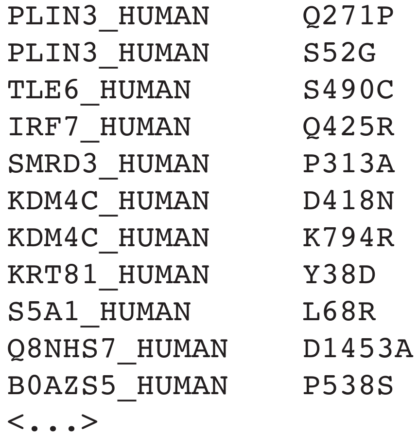
What is the SMLF file?

The idea of the simple mutation list format (SMLF) is to have a file format, which provides the information of mutations and their respective proteins while being as simple as possible. A SMLF file is a tab separated value file with only two columns. The first column contains the Uniprot entry name of the protein. (warning: do not confuse them with the Uniprot accesion number). The second column contains the amino acid variance in the following format: [one-letter code of the wildtype amino acid][position of the mutation in the amino acid sequence of the protein][one-letter code of the new amino acid]. For example: V302D

Example SMLF file:

What do the different output options?

When one uploads a job all given mutation datasets will be analysed once by the pipeline and the result will be stored in the MySQL database that connects all informations produced by the pipeline for at least one week. The initial analysis may take some time (typically, 40 mins for 1000 nsSNPs), so it is recommended to provide an email address to access the results later. The different outputs will be generated from these data and so choosing additional output options will not increase the running time significantly. By that we recommend always choosing at least the Annotation Output.

Annotation output

The annotation output lists all produced structural annotations and contacts, and allows to visually inspect position of each nsSNP in the corresponding 3D structures in a separate window. For each position of a nsSNP, the following information is displayed:

• Protein
  displays the Uniprot-ID of the protein harbouring the nsSNP.
• Structure
  displays the PDB-ID of the 3D structure used for the structural annotation of the nsSNP.
• Mutations
  displays all amino acid variants for the position provided in the input dataset.
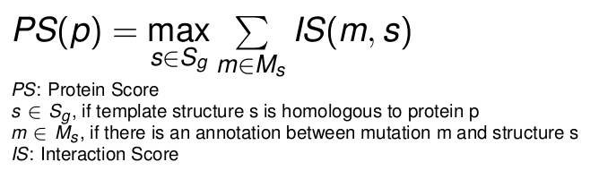
• Score
  The interaction score is the product of the structure quality score and the annotation candidate score. The interaction score displays the potential impact of the substitution corresponding to the nsSNP on the protein interactions. By default, the output list is sorted by this score.
• 3D-Viewer
  This button opens a new tab in your browser and loads the 3D structure of the protein or the protein homolog. In the structure, the residue corresponding to the nsSNP is shown in a balls-and-sticks style, while the surrounding protein chains are displayed as cartoons. The distances to all interaction partners are displayed.

Proteinsort output

This option allows the sort the output by the cumulative interaction score for all nsSNPs in a specific protein. That allows to select proteins with many high impact mutations.

• Protein
  displays the Uniprot-ID of the protein harbouring the nsSNP.
• Score
  This protein specific score is computed by finding the homolog structure with the highest cumulative sum of interaction scores, which are assigned to the nsSNPs of the protein.
  
  

GO term analysis

In the GO term analysis, all proteins from the input are grouped according to their GO terms. The GO term specific groups are then scored by the sum of their protein scores (see Proteinsort output), normalized by total number of proteins of the input set. This analysis reflects the overrepresentation of critical mutations in proteins with a certain biological function, process or localization. Given that there might be a natural bias in the input dataset, for a more clear picture one might prefer to perform a differential GO term analysis of a given input set versus a reference data set.

Differential GO term analysis

For this analysis, the user has to upload exactly two input data sets. The server performs the simple GO term analysis on both sets and then compares the results to each other. The output is sorted by the difference of the GO term scores of the GO terms that appear in both sets. The absolute value of the GO term score is not displayed, thus allowing to study the relative overrepresetation of certain GO terms corresponding to the mutations. If the difference is positive, the corresponding GO term is overrepresented in the first dataset, and vice versa.

Pathway analysis & Differential pathway analysis

The (differential) pathway analysis is similar performed as the (differential) GO-Term analysis, but the the proteins are grouped according to the pathways of the Reactome Database.

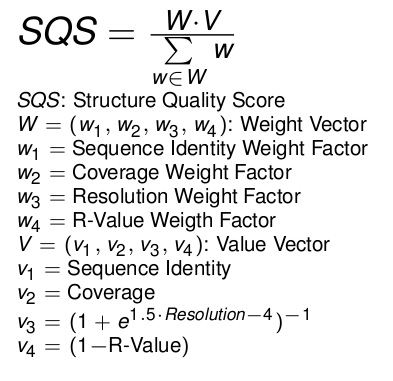
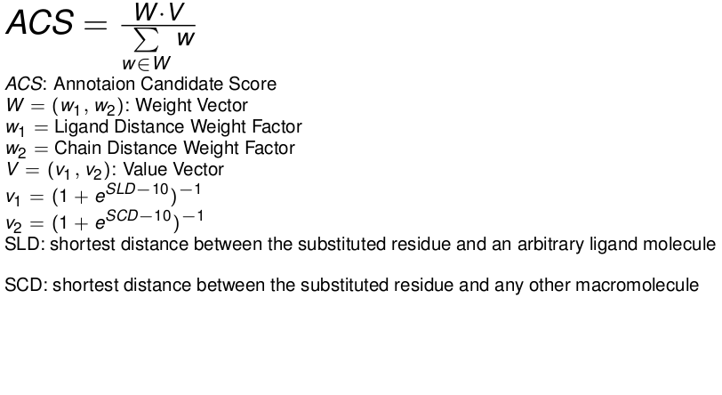
How are the scores computed?

The scores are linear combinations of a weight vector and a value vector and are normalized by the sum of all weight factors. The weight factors are an opportunity for the user to balance the scoring after his own intentions.

Example 1

For the structure quality scoring you want just consider the sequence identity and the coverage and decide, that the sequence identity is three times more important than the coverage. In this case you would set:

• Sequence Identity Weight Factor = 3
• Coverage Weight Factor = 1
• Resolution Weight Factor = 0
• R-Value Weight Factor = 0

Example 2

For the annotation candidate score you only want to consider contacts between the substituted residue and low molecular weight molecules. In this case you would set:

• Ligand Distance Weight Factor > 0
• Chain Distance Weight Factor = 0

Structure quality score

Annotation candidate score

Interaction Score

The interaction score is the product of the structure quality score and the annotation candidate score. It combines the structural informations of the residue position with reliability given by the structure quality.

What is a specified ligand analysis?

The specified ligand analysis enables the user to identify mutations, which are in contact to certain ligand molecules or to a certain class of ligand molecules. For the specified ligand analysis, the user has to provide a file with a list of low molecular weight ligands. The file can be in any format readable by the OpenBabel toolkit. The extension of the uploaded ligand file must correspond to the file format, as required by OpenBabel. The popular formats are: *.smi (SMILES), *.sdf (Structure Data File), *.mol2 (MOL2) or *.inchi (IUPAC INCHI Format). Additionally, the user has to provide a Tanimoto distance threshold. The pipeline finds all ligand molecules, which are similar enough according to the chosen threshold to the given molecules in the HETATM entries in all PDB files, and checks their distances to the mutations given in the mutation input dataset. The output will be sorted according to the similarity and the distance.

Options:

The options can be set after pressing the Show Options button on the upload page.
The options of StructMAn can either affect the selection of the homologous proteins with resolved 3D structures by the pipeline or the scoring function (and by that the sorting order of the produced outputs). One can generally say, that the more one restricts the template structure selection, the fewer nsSNPs will be structurally annotated, and fewer structures will be considered for annotation of a single nsSNP. The runtime also gets shorter and the output potentially more reliable. We do not recommend to restrict the template structure selection more than the default parameters, but relaxing these parameters may allow to identify more distant homologs with experimentally resolved 3D structures.

Input size dependent template filtering

This option reduces the number of templates used for the analyses. The amount of reduction is based on the number of given mutations. The reduction goes never below ten template structures per target protein. The reduction starts at input sizes of one hundred mutations and doubles with every order of magnitude. An input of 1.000 mutations is reduced by 50%, an input 10.000 is reduced by 75%, and so on.

Sequence identity threshold:

The sequence identity threshold restricts the template structure selection of the pipeline to pick structures with a sequence identity of the local pairwise amino acid sequence alignment of the template structure with the given protein.

Coverage threshold:

The coverage threshold is another filter based on the alignment between the homologous protein and the given protein. The coverage is the ratio between the length of the local pairwise sequence alignment and the length of the amino acid sequence of the protein.

Resolution threshold:

The resolution of the 3D structure of the homolog is a good measure of the overall quality of the experimental 3D structure. The value is given in angstrom.

Weight factors:

The weight factors balance the different sub-scores described in the scoring section.